Markov Games, Backwards Induction & Coordination Mechanisms

RL and Game Theory

Single-agent reinforcement learning works under a simple however important assumption: the environment is stationary.

In other words, the world behaves in a predictable way that depends only on the actions of a single learner.

In multi-agent systems conversely — which are prevalent in almost all real-world use cases, everything changes. Now each agent’s decisions directly influence what the other agents observe, the rewards they receive, and even how the environment evolves from one moment to the next.

From any single agent’s perspective, the environment is no longer stationary — it continues shifting because the other agents are also learning and adapting their behavior in real time.

This interdependence breaks the core assumptions of the Markov Decision Process (MDP) that classical single-agent reinforcement learning relies on.

Game theory, then naturally emerges as the ideal mathematical framework for understanding these more complex strategic interactions. It gives us the rigorous tools to analyze joint decision-making, equilibrium behavior, and the incentive structures among agents that may be self-interested, cooperative, or somewhere in between.

This study of strategic interaction was originally formalized by John von Neumann and Oskar Morgenstern in the 1940s and later significantly advanced by John Nash in the 1950s.

Its core concepts — especially the Nash equilibrium, best-response dynamics, and various cooperative and non-cooperative solution methods, become essential in multi-agent reinforcement learning (MARL).

Without these findings, MARL algorithms risk unstable training, suboptimal convergence, or simply failing to account for the strategic incentives that arise when numerous intelligent agents interact.

This publication is about multi-agent reinforcement learning (MARL) and how the Markov Game, also known as a stochastic game, provides the mathematical bridge between reinforcement learning and game theory. It explains how multiple intelligent agents make decisions in shared environments, how their actions jointly shape outcomes, and why concepts like reward functions, transition probabilities, finite versus infinite horizons, backward induction, Nash equilibrium, Pareto optimality, and different game types matter so much. By walking through cooperative, competitive, and mixed-agent settings, the post helps readers understand why MARL is becoming important in modern science, from robotics and climate modeling to quantum systems, drug discovery, and complex autonomous experimentation.

MARL in Modern Science and the Markov Game

In modern science, MARL is driving some of the most remarkable breakthroughs at the highest levels. It powers advanced multi-agent simulations for protein-protein interaction modeling in drug discovery, enables distributed control of quantum sensor networks, optimizes large-scale climate models through cooperative ensembles of agents, and facilitates autonomous experimentation in high-energy physics (like the tokamak) and synthetic biology.

"Give me a reward function, and I shall move the world." — Dr. Jim Fan, senior AI researcher at NVIDIA

So what serves as the natural bridge between reinforcement learning and game theory?

It is the Markov Game, also known as a stochastic game. This framework acts as the foundational mathematical structure for nearly all of multi-agent reinforcement learning.

A Markov Game generalizes the single-agent Markov Decision Process (MDP) to environments that involve many agents. In a standard MDP, one agent interacts with an environment defined by a state space, an individual action space, transition probabilities, and a reward function.

In a Markov Game, these core elements are extended to account for the presence and simultaneous decision-making of other intelligent agents.

In a Markov Game, these elements are extended as follows:

• First, there is a shared state space — just like in a single-agent MDP. The environment has one global state that evolves over time, and every agent can (in principle) observe aspects of it. However, in many realistic settings the agents only get partial observations.

• Second, instead of a single agent having its own action space, we now have a joint action space. Each agent still chooses its own action from its individual action space, but the overall action taken by the entire group is the combination of all those individual choices. This joint action is what drives the environment forward.

• Third, the transition probabilities now depend on the joint action of all agents, not just one. In other words, what happens next in the environment is shaped by what everyone decides to do simultaneously. This creates the non-stationarity we talked about earlier — the world looks different to you depending on how the other agents are behaving and learning.

• Finally, each agent has its own reward function. Unlike a single-agent MDP where there is one universal reward signal, a Markov Game gives every agent its own reward at each step. These rewards can be fully cooperative (everyone gets the same reward), fully competitive (one agent’s gain is another’s loss), or somewhere in between — creating the rich strategic dynamics that game theory was designed to analyze.

Putting it together, a Markov Game is defined respectively by this extended tuple:

𝐺 = (𝑆, 𝐴, ℙ, 𝑟, 𝛾, 𝜇)

• S is the shared state space,
• A is the individual action spaces, which together form the joint action space
• P is the joint transition probability
• R is the collection of individual reward functions for each agent
• γ is the discount factor (defining the present value of future rewards)
• 𝜇 is the initial state distribution.

At each time step, every agent selects an action simultaneously, the environment transitions to a new state according to the joint action, and each agent observes its individual reward and the next state. This structure captures the precise arena in which MARL algorithms learn.

Finite-Horizon vs. Infinite-Horizon Markov Games

Now that we’ve laid out the basic building blocks of a Markov/stochastic Game, there’s one more important distinction we need to make — and it has a big impact on how agents actually learn and behave.

Markov Games (and the multi-agent reinforcement learning algorithms built on them) come in two main flavors: finite-horizon and infinite-horizon. The difference is simple on the surface level, but it changes everything about the math, the strategy, and the kind of behavior that can emerge.

In a finite-horizon Markov Game, the interaction has a clear, fixed ending point. The game lasts for a known number of time steps — let’s say T steps, and then it stops. Every agent receives rewards along the way, and the goal is simply to maximize the sum of all those rewards from the very first step until the final step T. There’s no need for discounting because the game is guaranteed to end.

Think of it like a soccer match that lasts exactly 90 minutes, or a multi-agent robotics task that runs for a fixed number of seconds before the episode resets. Everything is time-limited, so agents can (in theory) plan ahead with perfect foresight about how many moves are left. This makes the problem episodic and often easier to analyze, when you’re dealing with short or medium-length tasks.

In contrast, an infinite-horizon Markov Game has no predetermined end. The interaction could, in principle, go on forever. Because an infinite sum of rewards would blow up to infinity, we introduce the discount factor (usually called γ, where 0 < γ < 1). This discount factor makes future rewards count less and less the further into the future they are.

It’s like saying, “A reward tomorrow is worth a bit less than a reward today, and a reward next month is worth even less.”

This version is perfect for continuing tasks where agents live in the environment indefinitely — think of autonomous traffic networks, ongoing economic markets, or persistent video-game worlds. The discount factor also has a nice side effect: it encourages agents to care more about near-term rewards while still considering the long run, which helps keep the total expected value mathematically well-behaved.

So why does this distinction matter so much in multi-agent reinforcement learning?

In finite-horizon games, the optimal strategy can actually change as the end of the game gets closer (a phenomenon sometimes called the “end-game effect”). In infinite-horizon games, the optimal policy is usually stationary — meaning the best thing to do in a given state doesn’t depend on what time step you’re on, which makes learning more stable and easier to generalize.

Both types appear frequently in real MARL applications, and the choice between them shapes everything from how we define the value functions to which equilibrium concepts make the most sense.

We’ll see exactly how these two horizons affect the Bellman equations, the learning algorithms, and the kinds of cooperation or competition that can emerge — but we’ll get into those details a little later.

The End-Game Effect: Backward Induction and the Finite Prisoner’s Dilemma

One of the most fascinating things about finite-horizon Markov Games is how the known ending dramatically changes agent behavior — especially as the final steps approach. When agents know exactly when the interaction will stop, their incentives shift. Future consequences disappear, so the pressure to cooperate or maintain good relationships with the other agents weakens.

To solve these games optimally, game theorists use a powerful method called backward induction. The idea is simple: start at the very last time step (when there is no future left and the game is basically a one-shot interaction), figure out the rational action there, then work backwards one step at a time to determine the best actions earlier in the game. This approach guarantees finding the subgame-perfect equilibrium.

A classic example that illustrates this is the finite repeated Prisoner’s Dilemma. Imagine two agents playing the Prisoner’s Dilemma for a known, fixed number of rounds — say 10 rounds. Even though both would be much better off if they cooperated throughout, backward induction reveals a interesting (and somewhat pessimistic) result: perfectly rational agents will defect in every single round, including the very first one.

Here’s why it happens: In the final round, since there is no future punishment possible, each agent’s best move is to defect. Knowing this in advance, the same logic applies to the second-last round, then the third-last, and so on — until cooperation completely unravels right from the beginning.

This “unraveling” effect shows how the knowledge of a definite ending can destroy the kind of sustained cooperation that often emerges in infinite-horizon settings. Keep this in mind as see later how this insight shapes the design of multi-agent reinforcement learning algorithms and what happens when agents don’t know exactly when the game will end.

Solution Concepts from Game Theory

In Markov Games, figuring out what counts as a “good” or “desirable” outcome isn’t always obvious. That’s exactly where solution concepts from game theory step in — they give us clear mathematical rules for deciding when agents are behaving rationally or optimally together.

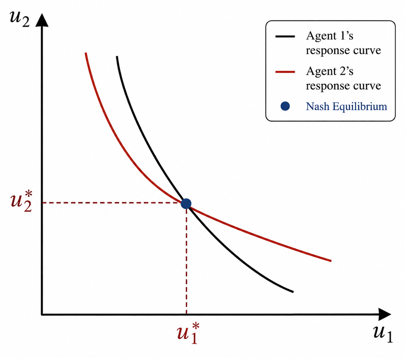
The most fundamental of these is the Nash Equilibrium. It’s a strategy profile (a set of policies, one for each agent) where no single agent can improve its own expected return by unilaterally changing its policy — as long as all the other agents stick to theirs.

In the world of MARL, a Nash Equilibrium acts like a stable resting point: once the agents’ learned policies reach it, nobody has any incentive to suddenly switch things up.

It's a natural balance.

However, actually finding a Nash Equilibrium in MARL is notoriously difficult. Non-stationarity, the explosion in joint action spaces (curse of dimensionality), and the fact that there are often many (often suboptimal) equilibria make it a formidable challenge.

Two other important concepts that often come up are Correlated Equilibrium and Pareto Optimality.

A correlated equilibrium relaxes the strict independence of the classic Nash idea. It lets agents coordinate their actions using a public signal or some kind of shared correlation device. This simple addition often unlocks higher collective payoffs than any pure Nash Equilibrium could achieve.

Pareto Optimality, on the other hand, describes a joint policy where no agent can improve its own reward without making at least one other agent worse off. It’s especially useful in cooperative settings because it focuses on overall social good.

Here’s the tension we often see in practice: MARL algorithms frequently settle into equilibria that are neither Pareto optimal nor correlated. The agents might reach a stable individual behavior, but the joint outcome can still be inefficient or far from what would be best for the group as a whole.

This is precisely why equilibrium selection and better coordination mechanisms remain some of the hottest areas of research in multi-agent learning.

We’ll dig deeper into how modern MARL algorithms try to steer agents toward better equilibria later on, as learning this will prove extremely useful within the near future with highly complex agentic systems.

Markov Games are typically categorized by the degree of alignment among agents’ objectives. This classification is critical because the nature of reward interdependence fundamentally shapes strategic behavior, learning dynamics, and the feasibility of cooperation or competition.

Types of Games in Multi-Agent Reinforcement Learning

One of the biggest factors that shapes which equilibria emerge, and how difficult they are to find — is the type of game the agents are actually playing. Markov Games can be broadly classified based on how the agents’ rewards relate to one another. We generally group them into three major categories: fully cooperative, fully competitive, and mixed (or general-sum) games.

Fully Cooperative Settings (Team Games)

In fully cooperative environments, all agents share the exact same reward function. Everyone wins or loses together, so individual interests and collective interests are perfectly aligned. These are often called team games. Success depends entirely on strong coordination between the agents.

Classic examples include robotic swarms working together to explore an unknown area or networks of sensors collaborating to provide optimal coverage. Because there is no conflict of interest, methods like value decomposition and centralized training with decentralized execution (CTDE) tend to work very well here. The main difficulties come down to credit assignment and effective coordination rather than fighting over conflicting goals.

Fully Competitive Settings (Zero-Sum Games)

At the opposite extreme are zero-sum games. In these environments, one agent’s gain is exactly equal to another agent’s loss — the total reward across all agents always sums to zero. This creates pure adversarial interactions.

You see this in classic two-player games like Go or chess, or in security scenarios with an attacker and a defender. In zero-sum games, the Nash equilibrium corresponds to the minimax solution, and training often leads to very robust, adversarial policies. While these settings offer strong theoretical guarantees, they can also produce highly conservative strategies.

Mixed or General-Sum Games

Most real-world multi-agent problems fall into the mixed, or general-sum, category. Here, the agents’ interests are neither fully aligned nor completely opposed. Rewards can sometimes be positively correlated (encouraging cooperation) and sometimes negatively correlated (encouraging competition), depending on the actions taken.

These environments are the most realistic — and often the most complex. Well-known examples include:

• The Prisoner’s Dilemma, where mutual cooperation is best for everyone, but each agent has a strong temptation to defect.
• The Tragedy of the Commons, where multiple agents over-exploit a shared resource, ultimately hurting everyone.
• The Stag Hunt, where agents must choose between a safe individual action or a high-reward option that requires trust and coordination with others.

In general-sum games, MARL systems have to carefully balance individual rationality with collective welfare. These settings frequently produce some of the richest emergent behaviors — things like negotiation, deception, and spontaneous cooperation — but they also create major challenges around equilibrium selection and training stability.

Conclusion

We’ve covered a lot of ground together. It has become clear that multi-agent reinforcement learning (MARL) is far more than just “RL with extra agents.”

In blending reinforcement learning with the strategic insights of game theory, MARL gives us a robust framework for understanding and designing intelligent systems that can coordinate, compete, cooperate, and even deceive in ways that feel remarkably human.

The emergent behaviors we can see, from spontaneous teamwork to sophisticated negotiation, show just how much social complexity can arise from simple reward signals and local learning rules.

As real-world applications continue to explode, from drug discovery and climate modeling to autonomous robotics and beyond — the ability to reliably guide multi-agent systems toward stable, efficient, and socially desirable outcomes will only become paramount to achieve success in this period.

In the posts ahead, we’ll dive deeper into the algorithms, the math, and the practical techniques that make all of this possible. For now, I hope this overview has given you a clear sense of why MARL sits at such an exciting intersection of artificial intelligence and game theory, and why it’s one of the most promising frontiers in AI today.

Thanks for reading, and I’ll see you in the next publication.