Memoryless: Hidden Markov Models in Machine Learning (part 2)

Machine Learning is not about machines becoming intelligent. It's about machines helping us see patterns we were never equipped to see

Sequential data surrounds all of us. Every spoken sentence, every strand of DNA, or sequences of market movements, all unfold over time according to patterns we cannot directly observe.

In these settings, the central challenge isn't as much the observation itself, but instead the latent (hidden) process that creates it. Hidden Markov Models (HMMs) provide a principled probabilistic framework for modeling this relationship between observable data and underlying, latent dynamics.

Long before deep learning architectures took over the field, HMMs powered large-scale speech recognition systems, bioinformatics (computational gene and protein structure prediction), and supported early advances in handwriting recognition systems.

Even today, they remain important conceptually: many contemporary models either expand or reinterpret the assumptions first formalized in the HMM framework.

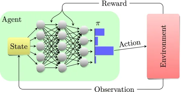
Making it clear, HMMs don't follow the same dynamics that Reinforcement Learning frameworks follow. There is no mention of actions or rewards, instead they follow a passive stochastic process. Indeed, HMMs originate from the world of Machine Learning and Probabilistic modeling. However, they are structurally closely related to the Partially Observable Markov Decision Process, which is briefly mentioned here. An HMM can be viewed as a special case of a POMDP in which no actions are taken and no rewards are defined. POMDPs further the HMM framework by introducing control (actions) and optimization (rewards) on top of the same latent-state and observation structure. Many reinforcement learning methods under partial observability rely on latent state inference mechanisms that are conceptually rooted in HMMs, making this connection fundamental.

At the substrate of HMMs, they formalize the idea:

An observed sequence is generated by an underlying sequence of hidden states that evolve according to Markovian dynamics.

The system transitions between latent states over time, and each state emits observations according to a probability distribution. The states themselves are not directly observable — only their emissions are.

The task, therefore, is of statistical inference: recovering information about the unknown state trajectory and model parameters from noisy and incomplete observations.

Let's provide an example, consider automatic speech recognition. When a person speaks into a device, like Siri back in the day when it primarily used HMMs, the raw audio waveform was segmented into short time frames.

From each frame, instead of the words you used, only basic features are extracted — the speech volume, spectral coefficients, pitch-related information, and so on. To the machine these features do not directly represent linguistic units such as phonemes; instead, they are just signals that hint at what might have been said, using probability. It works backwards to understand you.

As a result a HMM models speech as a sequence of hidden linguistic states, each evolving according to transition probabilities that encode how likely one sound is to follow another. Each hidden state (words you spoke) generates acoustic observations according to an emission distribution. This distribution is what then links sound to signal — the system now understanding and acting on your request.

By modeling this, HMMs provide a tangible way to reason about temporal uncertainty (the uncertainty as to how systems evolve through time).

Given only what we can observe, what can we infer about the underlying structure we cannot see?

To now formalize the discussion, we move from intuition to the mathematical structure of a Hidden Markov Model. An HMM is a generative probabilistic model defined by three fundamental components:

• The initial state distribution (π)
• The transition probabilities (A)
• The emission (observation) probabilities (B)

Together, these define a complete joint distribution over hidden and observed sequences.

π is simply a matter of notation reuse, not to be confused with the policy from RL.

1. Hidden and Observable States

An HMM consists of two coupled stochastic processes:

• A hidden state sequence:

$X_{1:T} = (X_1, X_2, \dots, X_T)$

• An observable sequence:

$Y_{1:T} = (Y_1, Y_2, \dots, Y_T)$

At each time step t:

• $X_T$ represents the latent state of the system.
• $Y_T$ represents the observable output generated from that hidden state.

For simplicity, consider a binary-state example — remember ∈ is denoted as "is an element of." I will also be adding more binary-state examples in the near future for the next sections.

• Hidden states: $X_t \in \{x_1, x_2\}$
• Observations: $Y_t \in \{y_1, y_2\}$

Again, the hidden states $X_T$​ are not directly observable. Instead, we only observe $Y_T$, which is probabilistically dependent on $X_T$.

2. The Initial Distribution

The model begins with a probability distribution over the initial hidden state:

$\pi_i = P(X_1 = x_i)$

For the two-state case:

$\pi_1 = P(X_1 = x_1)$, $\pi_2 = P(X_1 = x_2)$

with:

$\pi_1 + \pi_2 = 1$

This distribution encodes prior belief about the system’s starting configuration.

3. Transition Probabilities

The hidden states evolve according to the Markov property, meaning:

$P(X_t \mid X_{t-1}, X_{t-2}, \dots) = P(X_t \mid X_{t-1})$

Thus, the future depends only on the present state, not the full history.

The transition probabilities are defined as:

$a_{ij} = P(X_t = x_j \mid X_{t-1} = x_i)$

4. Emission Probabilities

The observable variable $Y_t$ depends only on the current hidden state $X_t$​. This is the conditional independence assumption central to HMMs:

$P(Y_t \mid X_1, \dots, X_t, \dots) = P(Y_t \mid X_t)$

The emission probabilities are defined as:

$b_j(k) = P(Y_t = y_k \mid X_t = x_j)$

5. The Generative Structure within a HMM

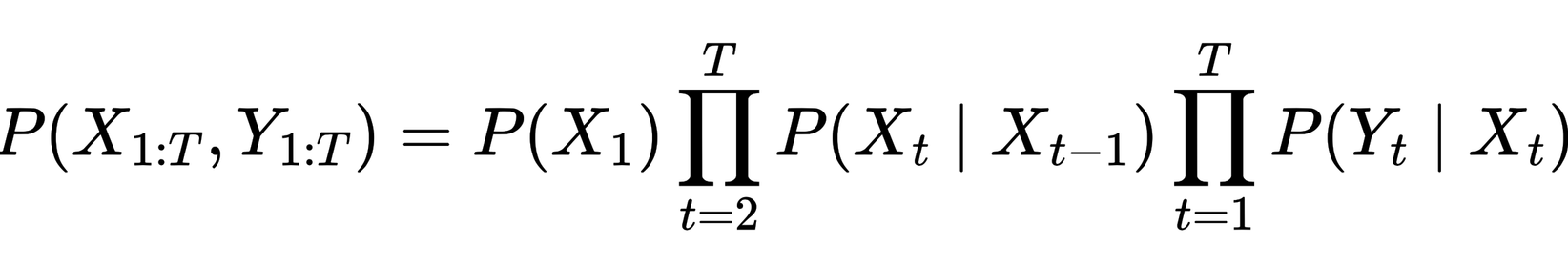
With these components, the joint probability of a hidden sequence $X_{1:T}$ and observation sequence $Y_{1:T}$ factorizes as:

A side-note, if you find yourself confused, I will be adding to this section to allow full understanding within the next few days.

This factorization reflects the two structural assumptions:

1. Markovian state evolution
2. Conditional independence of observations given states

This expression defines the joint probability of the hidden state trajectory and the observed sequence, and follows directly from the Markov and conditional independence assumptions of the model.

Interpretation

Conceptually:

• The initial distribution determines where the process starts.
• The transition matrix governs how the hidden system evolves.
• The emission model explains how hidden structure manifests in observable data.

From this foundation, we can then proceed to the central inference problems of HMMs like:

• Evaluating sequence likelihoods
• Decoding the most probable state path
• Learning parameters from data

Each of these rests directly on the mathematical structure introduced in this post.

From Structure to Inference

With the structural components of the Hidden Markov Model now formalized — the initial distribution, transition dynamics, and emission mechanism, we have defined a complete probabilistic generative model. But specifying the model is only the start. The real substance of HMMs lies in what they allow us to compute.

Once the triplet (π, A, B) is established, three fundamental inference problems emerge:

• Evaluation – Given an observed sequence $Y_{1:T}$ what is its likelihood under the model?
• Decoding – What is the most probable hidden state sequence $X_{1:T}$ that could have generated the observations?
• Learning – How can the parameters (π, A, B) be estimated from data when the states themselves are unobserved?

These are inferential questions at the crux of probabilistic modeling. They transform the HMM from just a descriptive structure into an operational framework for reasoning under uncertainty.

The beauty of the HMM lies in the fact that each of these problems admits principled solutions grounded in dynamic programming and probabilistic recursion:

• The Forward algorithm enables tractable computation of sequence likelihoods.
• The Viterbi algorithm identifies the most probable latent trajectory.
• The Baum–Welch algorithm allows parameter learning in the presence of hidden variables.

What initially presents as an inference problem of exponential complexity becomes tractable through the conditional independence structure and first-order Markov assumptions encoded in the model. These structural constraints permit efficient recursive computation without enumerating all possible latent trajectories. It is precisely in this disciplined balance between abstraction and structure that the strength of Hidden Markov Models emerges.

"What I cannot create, I do not understand." — Richard Feynman

Looking Ahead

In the next part, we will move from structural formulation to operational inference. We will begin by deriving the forward recursion for evaluating sequence likelihoods, examine why naïve computation is impossible, and show how dynamic programming resolves this efficiently.

From there, we'll explore decoding and parameter estimation, building toward a complete inferential equipment set for Hidden Markov Models.

The foundational framework is now in place. What will follow is where the mathematics becomes complete.

I will be modifying this post as time goes on, so if you find yourself confused, especially by the math, feel free to send me an email:

leon.axel9821@gmail.com