π: What it is in Reinforcement Learning
Reinforcement learning (RL) is one of the most exciting areas of artificial intelligence today. Deriving from behavioural psychology, particularly the concepts of operant conditioning and trial-and-error learning, RL at its essence is about teaching an AI agent to align with a goal via sequential decisions that lead to the highest reward over time.
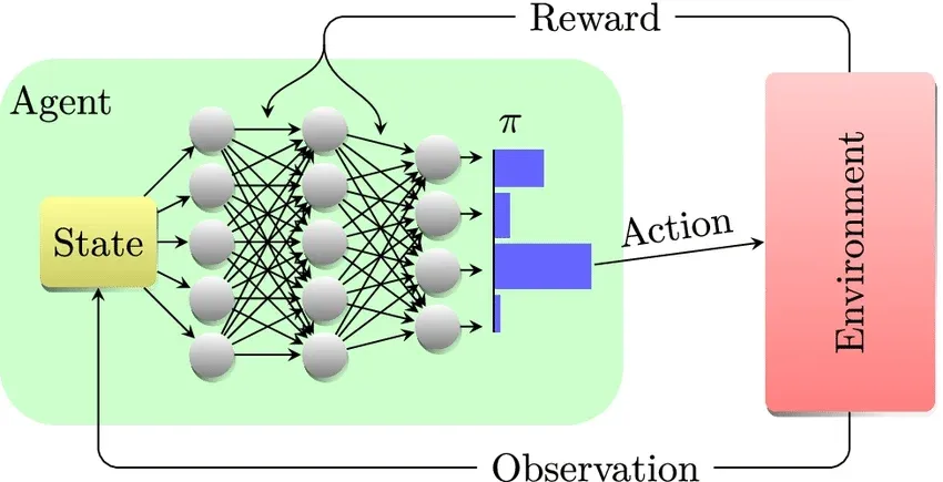
We will be discussing the policy, denoted π — the strategy that defines how an agent behaves based at a given point within the environment.
This is the primary goal of a reinforcement learning algorithm: to learn an optimal policy that maximizes the agent's total expected cumulative reward over time. Let's explore this further.
Our Track Record
To revise, in these previous posts on RL we’ve established a brief rundown of some foundational concepts that underlie optimized decision-making:
First we explored the Bellman Optimality Equation, which defines how to recursively calculate the maximum expected reward from any given state — helping to derive the optimal policy.
Recursive here refers to solving complex, long-term problems by breaking them down into smaller, self-similar sub-problems, typically using feedback loops where the output of one step becomes the input for the next
So, while the policy defines the agent’s strategy — how it chooses actions in each state, the Bellman optimality equation tells us how good each action is by evaluating the expected return. As a result this enables the agent to iteratively improve its policy, step by step, until it converges to the optimal one.
We then introduced Markov Decision Processes (MDPs) — a formal framework for sequential decision-making, often under uncertainty. An MDP is commonly defined by states (S), actions (A), transition dynamics (P), a reward function (R), and a discount factor (γ), and sometimes an initial-state distribution.
These ingredients let us fill in the blanks for the Bellman optimality equation. In model-based settings where the agent has or builds a map of the current state, where P and R are known or can be estimated, the optimality equation can be used for planning; in model-free settings where the agent has no idea where it is, algorithms still learn optimal values from experience without explicitly building the full model.
This is modeled using Partially Observable Markov Decision Processes (POMDPs), a mathematical framework for decision-making under uncertainty where an agent cannot directly observe the true environment state. Instead, the agent receives observations and maintains a probabilistic belief over possible states, selecting actions to maximize expected cumulative reward based on this belief.
Afterwards, we unveiled the Markov property, an assumption entrenched in Markov models such as MDP's and POMDP's which simplifies complex systems by ensuring that all relevant information from the past is captured in the present — a concept that allows models to efficiently make predictions, while avoiding state space explosions through the use of sufficient statistics.
Building on this, we examined Markov Chains, which provide the foundational mathematical framework for modeling probabilistic transitions between states, which is later extended by MDPs and POMDPs to include actions, rewards, and uncertainty in perception.
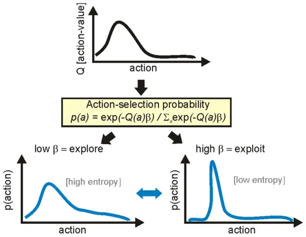
Last but not least, we discussed the exploration vs. exploitation trade-off — a key principle in reinforcement learning that ensures agents don’t just stick to what they know, but also take random or calculated risks to discover better long-term strategies.
This ultimately influences how a policy is shaped over time. An optimal policy balances both: it exploits known high-reward actions while still exploring enough to discover potentially better strategies.
Exploration mechanisms such as ε-greedy or softmax shape policy learning by trading off immediate exploitation against information gathering. While the Bellman equation defines the optimal value target, these strategies control how the agent samples actions to approximate that target, often gradually reducing exploration over time as estimates converge.
All together so far, these ideas are now forming a greater synergy for teaching machines how to learn, adapt, and make smarter decisions over time.
With this added clarity, let's dive into the landscape of policies.
The 2 Types of Policies and Examples
A policy is the agent’s core decision-making mechanism, defining how each state of the environment is mapped to an action. Effectively it tells the agent: “When you see this particular state, do this action."
There are two main types of policies:
- Deterministic Policy – This policy is a fixed rule that maps each state to a single, specific action, meaning there's no randomness in its decision-making; for any given situation (state), it always chooses the same action, making it predictable and useful for applications in industrial control. The deterministic policy is simply represented as a function π(s) = a, where state s leads to action a.
- Stochastic Policy – Outputs a probability distribution, the agent may select different actions with certain probabilities — the policy assigns higher probabilities to favourable actions, and vice versa. This is useful for more complex systems that have environments that require POMDP's or numerous agents (Multi Agent RL). The notation used is π(a|s), which represents the conditional probability of taking a specific action a, given a particular state s.
While π(a|s) is the most common, other equivalent or similar notations are also used.
A cool example regarding the stochastic policy is an agent that maps cell differentiation, the process where an immature, unspecialized cell like a stem cell transforms into a specialized cell type like a neuron or white-blood cell.
Using a single-cell RL framework, researchers treat cell differentiation as a partially observable, sequential decision process, where the agent learns a stochastic policy π(a|s) that maps observed cellular states to differentiation actions — helping us in understanding the stochastic nature of biological processes from the results of what the agent can infer from critical intervention points.
Current and traditional methods have a hard time pinpointing when cells make these complex inflection points, however with methods like single-cell RL, in understanding how cells develop into different types during growth and disease, scientists could guide stem cells into specific cell types and repair damaged tissues, and design treatment plans that step in precisely with the pathways that have gone wrong.
How Policies Are Learned
There are two common approaches:
1. Policy‑Based Methods
Policy-based methods, which are prominent in robotics, are approaches where the agent learns the policy directly, which means it learns how to choose actions from states without first learning a value table or score for each action. Instead of asking “how good is this action?”, the agent adjusts the decision-making rule itself so that actions leading to higher long-term rewards become more likely over time.
This is often done by slightly changing the policy after each episode or batch of experience in the direction that increases total reward, basing on what has worked best in the past.
2. Value‑Based Methods
Alternatively, value-based methods in reinforcement learning are approaches where the agent learns how good different states or actions are, rather than learning the policy directly. The agent estimates a value function that predicts the expected long-term reward from a state or from taking a specific action, and then chooses actions by selecting the one with the highest estimated value.
The best policy is then obtained by selecting the action with the highest Q-value in each state, which we'll delve into further. Instead of storing a policy explicitly, they use lookup tables (Q-tables) to assign values to state-action pairs (Q(s, a)).
To paraphrase the key points, policies are often derived by choosing, for each state, the action with the highest estimated Q(s,a). And value-based methods do not explicitly store or represent the policy — but they implicitly define one through the value function.
3. Actor-Critic Methods
Actor-critic methods bridge policy-based and value-based learning. They maintain two components:
- The actor, which learns and stores the policy directly and decides which actions to take.
- The critic, which estimates the value function to judge how good the actors actions are.
Both the actor and the critic maintain their own sets of function-based parameters. The critic evaluates the outcomes of the actor’s decisions and provides feedback, which the actor uses to update its policy. As with many AI systems, the dual structure allows for more stable learning.
Another cool fact, back in 2016 a subdivision of Google DeepMind, DeepMind Applied, developed an AI system that used Deep RL (including elements that function like an actor-critic model) to optimize the control of Google's data centre cooling systems, achieving an impressive 40% reduction in energy expenditures and a 15% reduction in overall Power Usage Effectiveness overhead.
The Soft Actor-Critic (SAC) and Proximal Policy Optimization (PPO) algorithms are well-suited for these types of data centre control problems.
Policies in Practice: On‑Policy vs Off‑Policy Learning
In reinforcement learning, on-policy and off-policy describe whether an agent learns from the same strategy it uses to act.
- On-policy learning means the agent improves the policy it is currently following. It learns directly from its own actions during exploration (for example, SARSA).
- Off-policy learning means the agent can learn one policy while behaving with another. This allows it to reuse old experiences or data collected with different strategies (for example, Q-learning).
On-policy learns only from what it does.
Off-policy learns from what it (or others) have done.
On-policy methods tend to be more stable but need fresh data, as they can only learn correctly from experiences generated by their current policy, once the policy changes, old data no longer matches how the agent behaves.
Off-policy methods are more sample-efficient because they can reuse past experience, but they can be harder to train reliably, because they learn from data generated by different behaviour than the policy they’re trying to optimize — this can create a mismatch that can destabilize learning.
Conclusion
Hopefully you found this post insightful and valuable for your journey, there are still tons of insights for on/off policy methods as well as Q-learning and SARSA algorithms that I would like to cover soon to add more intuition. For next post however, I’ll be adding a review for the business side of the blog — a standout episode from the Y Combinator podcast.
In that post I'll be discussing good wisdom on designing products that truly differentiate themselves from others, things that have proven invaluable in my own journey.
I hope everyone’s having a marvellous Christmas break so far. Happy holidays and I will be seeing you soon.